Examples¶

Your first bubble simulation

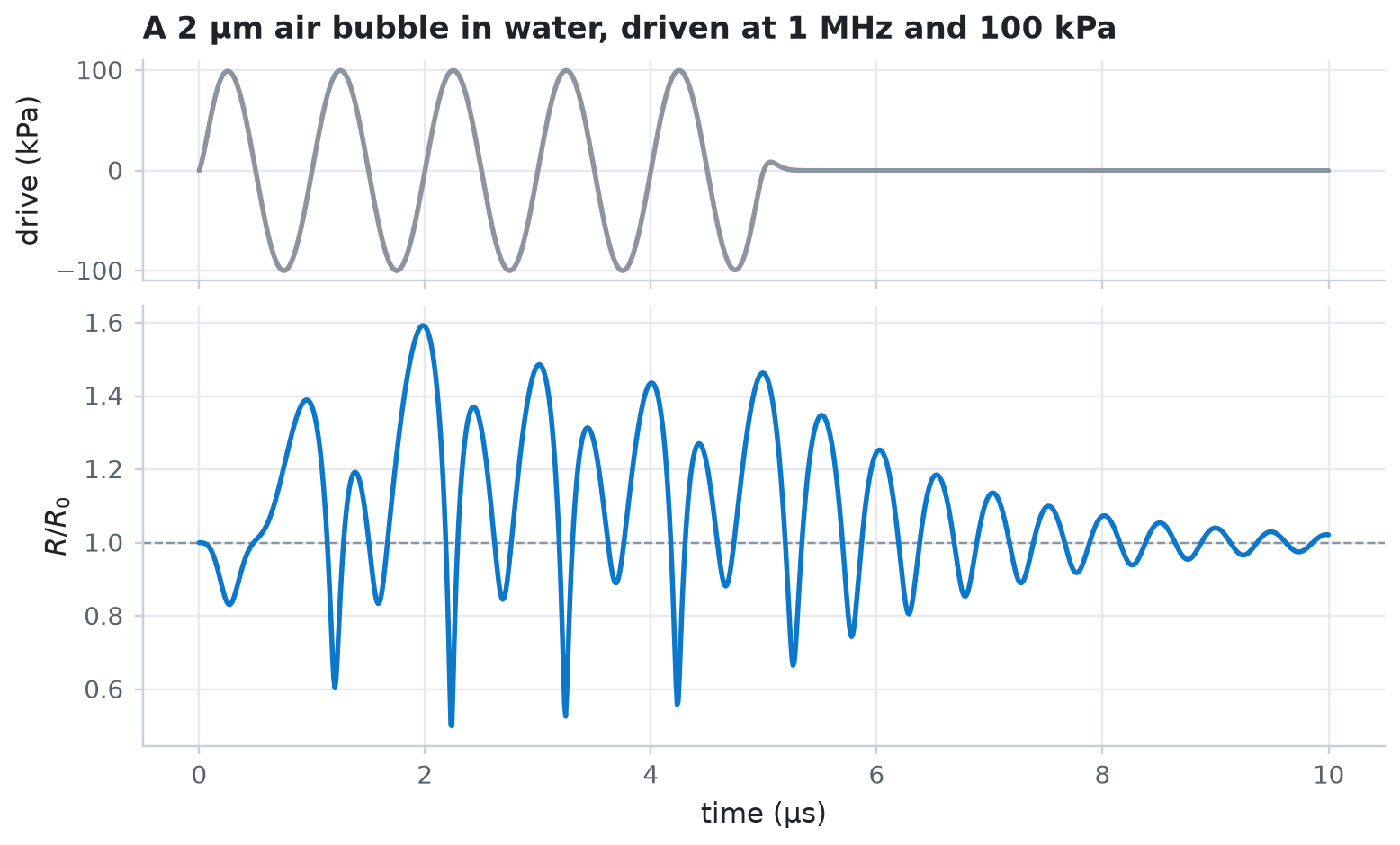
Simulate a gas microbubble driven by a short ultrasound pulse. You run a preset in five lines, build the same model from its parts, and then compile the simulation once so that every later run takes milliseconds.

Driving pulses

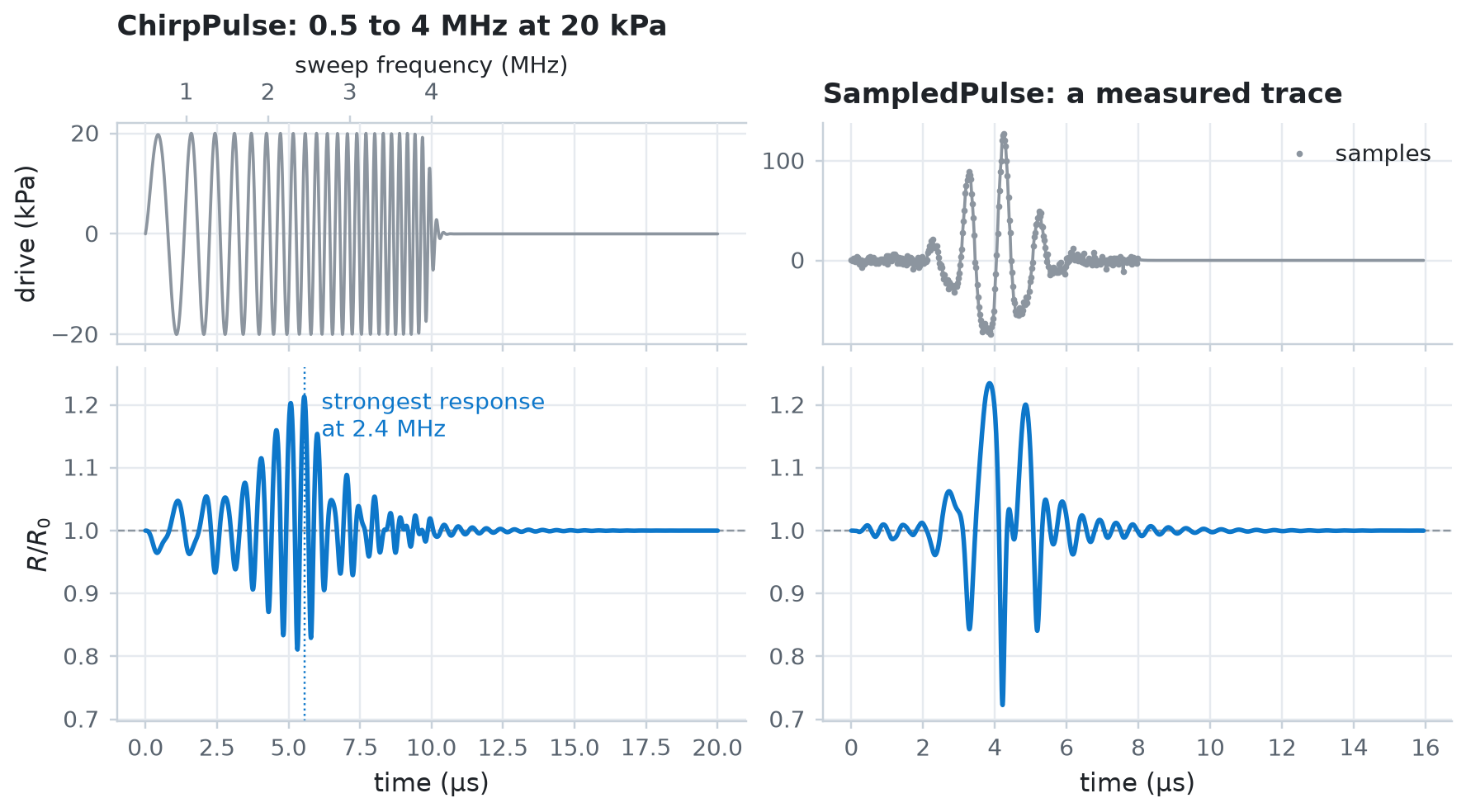
Shape the ultrasound that drives a bubble. You compare carrier shapes, combine pulses with arithmetic, sweep the frequency with a chirp, and load a pressure trace measured on a hydrophone. Then you drive the same bubble with the chirp and with the measured trace.

Shells, gases, and media

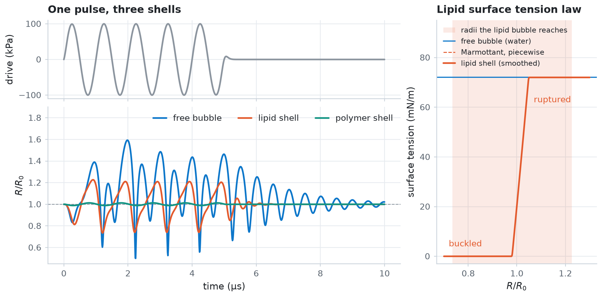
Compare the physical parts of a bubble model. You drive an uncoated bubble, a lipid-coated contrast agent, and a polymer-shelled agent with the same pulse, and you see how the lipid shell's surface tension changes with the radius. Then you swap the gas law and the surrounding medium.

Equations of motion

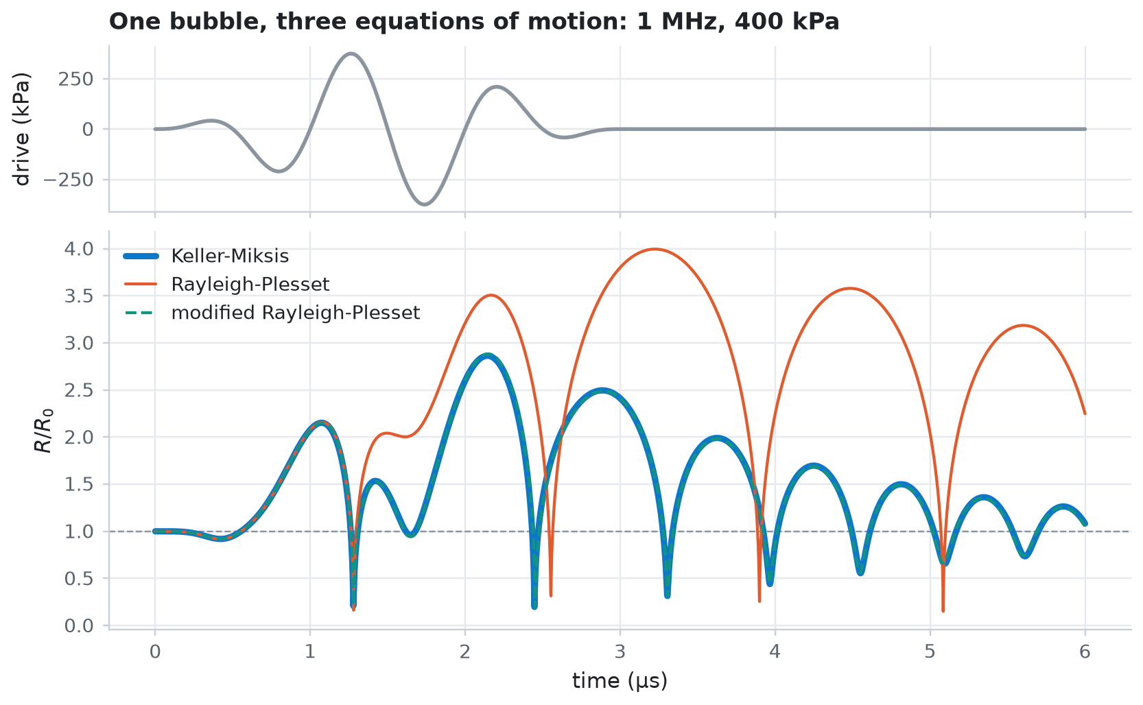
Solve one bubble with three equations of motion, from the incompressible Rayleigh-Plesset equation to the Keller-Miksis equation, which accounts for the compressibility of the liquid. Then raise the drive pressure to see where stable oscillation gives way to inertial cavitation.

Parameter sweeps

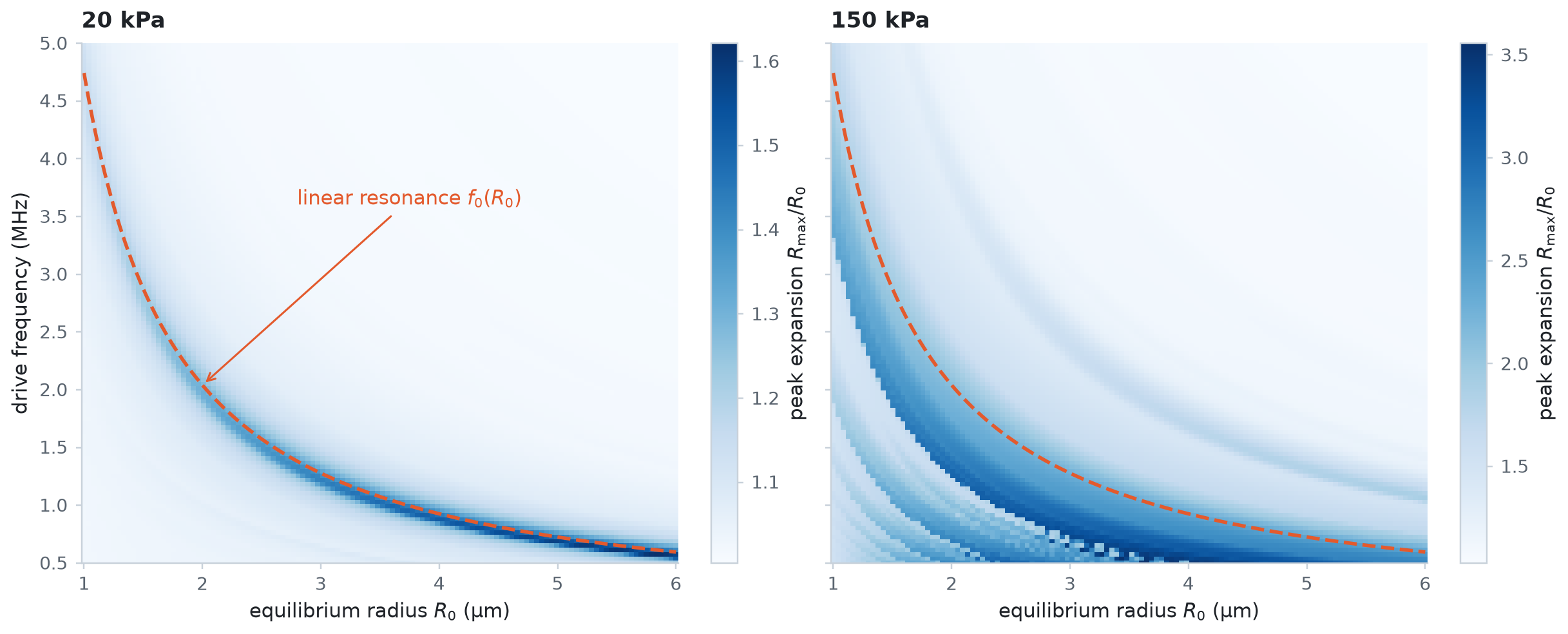
Run thousands of bubbles at once. jax.vmap simulates a row of bubbles of different sizes in one call, and GridSweep maps the response over a grid of radius, frequency, and pressure on every CPU core. The map is checked against linear resonance theory, collected batch by batch, saved to a NumPy file, and drawn from that file.

Acoustic emission

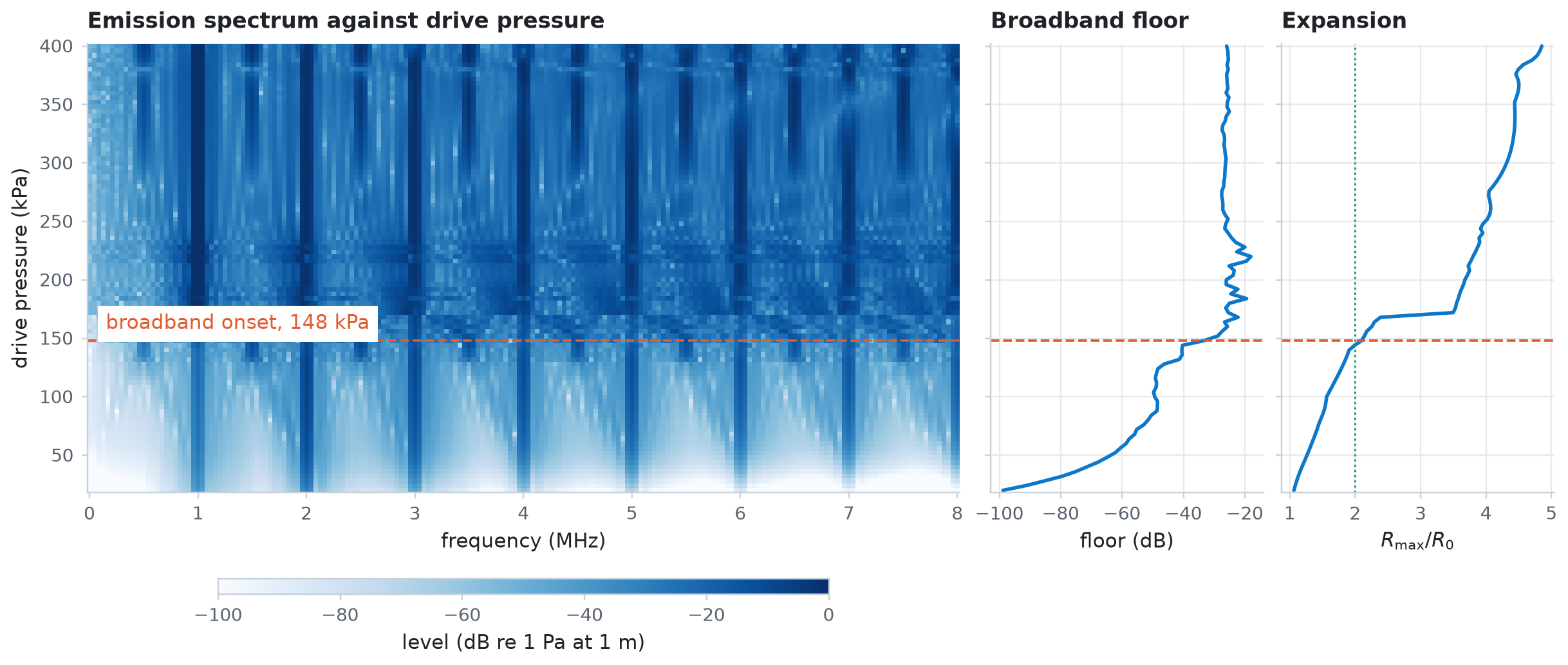
A hydrophone measures the pressure that a bubble radiates, not its radius. Compute that pressure with IncompressibleMonopole and QuasiAcoustic, turn it into a Hann-windowed spectrum without aliasing, and map how the spectrum changes with drive pressure: harmonics at low pressure, then broadband noise once the bubble collapses inertially.

Solvers and stiffness

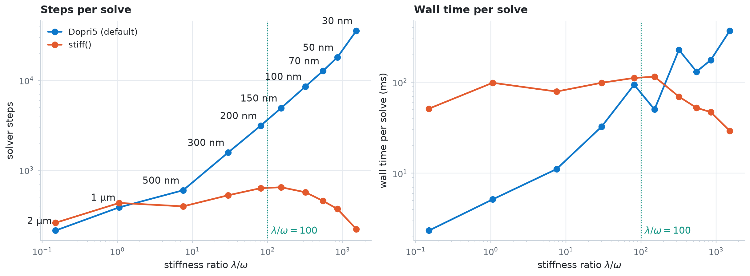
jbubble integrates with the explicit Dopri5 solver by default, which suits microbubbles. Small or viscous bubbles make the equations stiff. Measure where the implicit solver of SolverConfig.stiff() wins, see how max_steps and converged report a solve that runs out of steps, and see why a stiff problem needs the implicit solver for gradients.

Custom physics

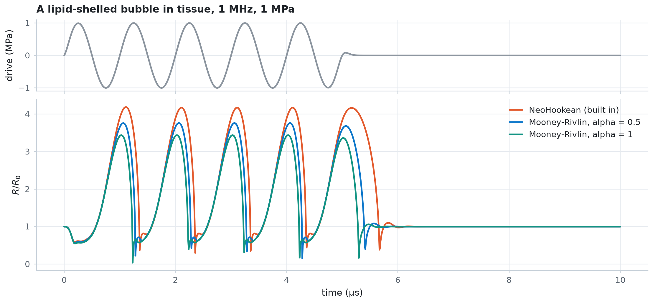
Add your own laws without touching jbubble. Subclass Property for a state-dependent coefficient, subclass MediumModel for a new surrounding medium, and plug both into KellerMiksis. Then replace a law that you don't know with a neural network through NeuralProperty, and differentiate a simulation with respect to its weights.

Gradients and optimisation

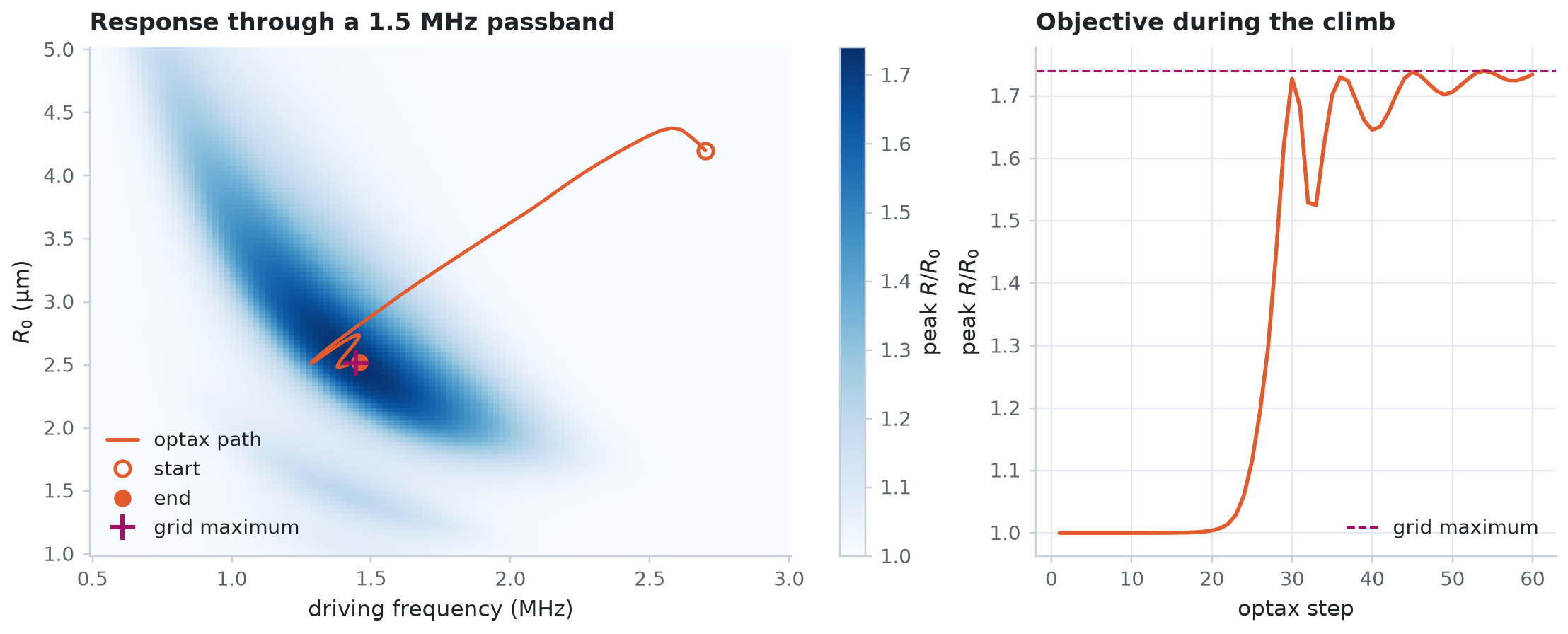
Every jbubble simulation is a JAX function, so jax.grad differentiates any scalar result with respect to any model input, straight through the ODE solve. In this example, you check a gradient against finite differences, compute a whole sensitivity curve in one jax.vmap(jax.grad(...)) call, and use the gradient to climb a response map with an optax optimiser.

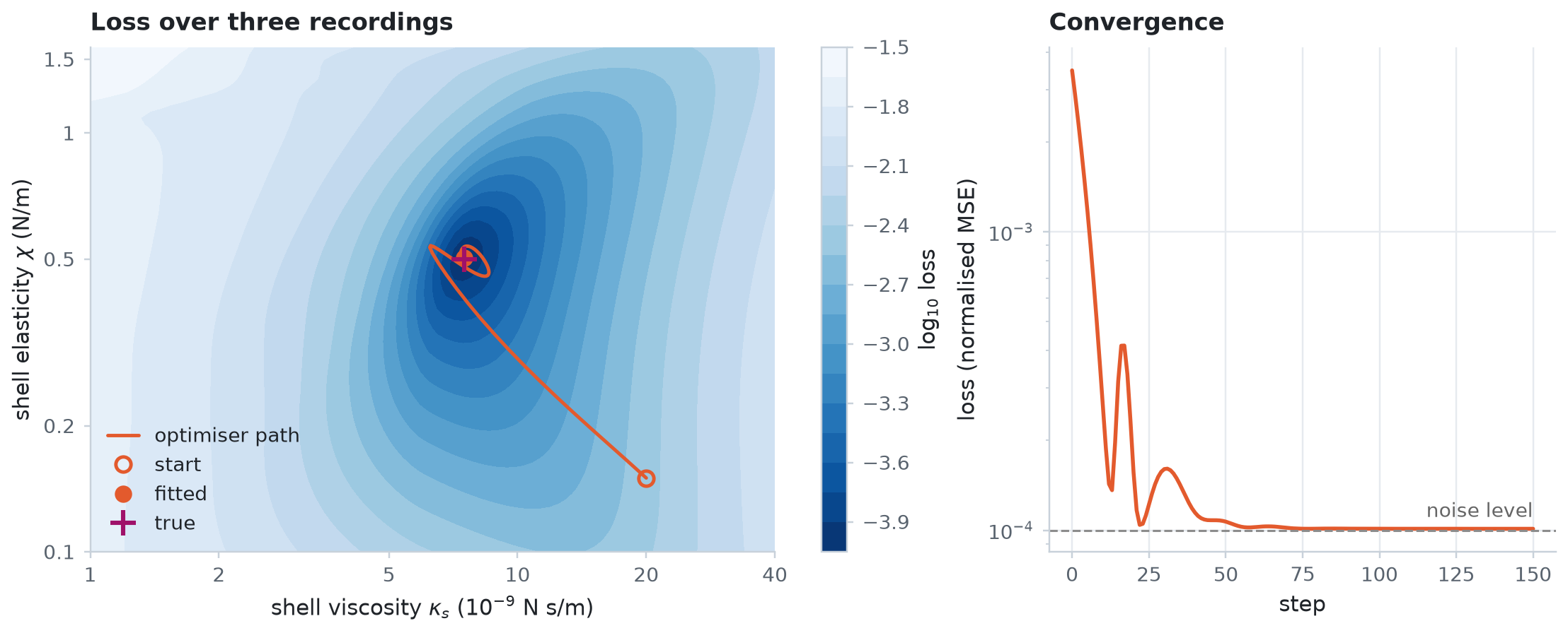
Fit shell parameters to radius curves

Estimate the elasticity and the dilatational viscosity of a lipid shell from noisy radius-time curves recorded at three driving pressures. In this example, you declare the unknowns with Parameter bounds, fit all three recordings at once with fit_parameters, and look at the loss landscape that the optimiser walks across.

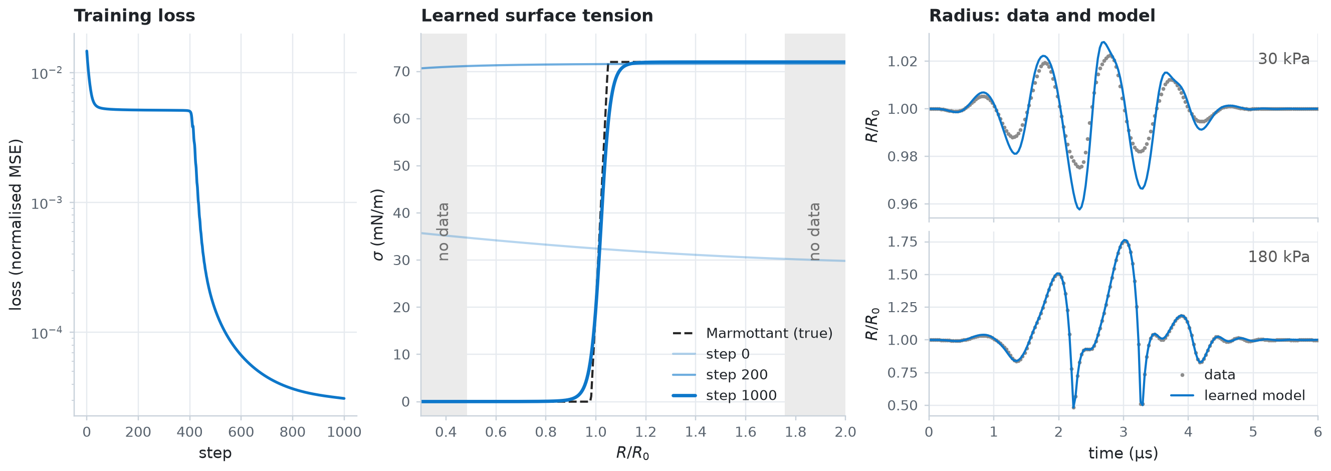
Learn a shell law with a neural network

When you don't know the form of a constitutive law, you can learn it from data. In this example, a small neural network takes the place of the surface tension \(\sigma(R)\) of a lipid shell, and fit_parameters trains its weights on radius curves recorded at six driving pressures. The network recovers the buckling, elastic, and ruptured regimes of the Marmottant law without being told that they exist.