Solvers and stiffness

jbubble integrates with the explicit Dopri5 solver by default, which suits microbubbles. Small or viscous bubbles make the equations stiff. Measure where the implicit solver of SolverConfig.stiff() wins, see how max_steps and converged report a solve that runs out of steps, and see why a stiff problem needs the implicit solver for gradients.
import os
import textwrap
import time
import warnings
from functools import partial

import diffrax
import jax
import jax.numpy as jnp
import matplotlib.pyplot as plt
import numpy as np

from jbubble import SaveSpec, SolverConfig, run_simulation, solve_eom
from jbubble.utils.presets import lipid_bubble

plt.style.use("jbubble.style.light")

# JBUBBLE_QUICK=1 shrinks the benchmark for continuous integration (CI).
QUICK = os.environ.get("JBUBBLE_QUICK", "0") == "1"
The default solver
SolverConfig() is an adaptive fifth-order Runge-Kutta method with a proportional-integral-derivative (PID) step-size controller. Its tolerances apply to the scaled state: the radius in units of \(R_0\) and the wall velocity in units of \(\sqrt{P_\text{amb}/\rho_L}\).
default = SolverConfig()
stiff = SolverConfig.stiff()
for name, config in [("SolverConfig()", default), ("SolverConfig.stiff()", stiff)]:
    controller = config.stepsize_controller
    print(
        f"{name:21s} {type(config.solver).__name__:8s} rtol={controller.rtol:g} "
        f"atol={controller.atol:g} max_steps={config.max_steps}"
    )
SolverConfig()        Dopri5   rtol=1e-06 atol=1e-10 max_steps=100000
SolverConfig.stiff()  Kvaerno5 rtol=1e-06 atol=1e-10 max_steps=100000
A stiffness ratio
A bubble is stiff when its fastest relaxation rate is much larger than the angular drive frequency \(\omega\). For a lipid shell with dilatational viscosity \(\kappa_s\) in a liquid of viscosity \(\mu\), that rate is about
where the denominator is the Keller-Miksis radiation correction. Both terms grow as the bubble shrinks, so nanobubbles are stiff even in water. Expect trouble for an explicit solver when \(\lambda/\omega \gtrsim 100\).
FREQ = 5e6  # drive frequency [Hz]
KAPPA_S, MU, RHO_L, C_L = 7.5e-9, 1e-3, 998.0, 1500.0  # lipid_bubble defaults


def stiffness_ratio(R0):
    damping = 4 * MU + 4 * KAPPA_S / R0
    rate = damping / (RHO_L * R0**2) / (1 + damping / (RHO_L * C_L * R0))
    return rate / (2 * np.pi * FREQ)


def solve(R0, config):
    """Solve a lipid bubble of radius R0 at 5 MHz and 100 kPa; return (ok, steps)."""
    eom, pulse = lipid_bubble(R0=R0, freq=FREQ, pressure=100e3, cycle_num=5)
    sol = solve_eom(eom, pulse, save_spec=SaveSpec(num_samples=256), config=config)
    return diffrax.is_successful(sol.result), sol.stats["num_steps"]


def wall_time(fn, *args, repeats):
    """Return the best of `repeats` wall times [s] after one warm-up call."""
    jax.block_until_ready(fn(*args))
    best = np.inf
    for _ in range(repeats):
        t0 = time.perf_counter()
        jax.block_until_ready(fn(*args))
        best = min(best, time.perf_counter() - t0)
    return best
Steps and wall time against stiffness
Solve the same lipid-shelled bubble, driven at 5 MHz and 100 kPa, at radii from 2 µm down to 30 nm, with both configurations. The radius is an argument of the compiled function, so each configuration compiles once.
radii = (
    [2e-6, 500e-9, 150e-9, 50e-9]
    if QUICK
    else [2e-6, 1e-6, 500e-9, 300e-9, 200e-9, 150e-9, 100e-9, 70e-9, 50e-9, 30e-9]
)
repeats = 1 if QUICK else 5
solvers = {
    "Dopri5 (default)": jax.jit(partial(solve, config=default)),
    "stiff()": jax.jit(partial(solve, config=stiff)),
}

ratios = np.array([stiffness_ratio(R0) for R0 in radii])
steps = {name: [] for name in solvers}
times = {name: [] for name in solvers}
print(" R0 (nm)  λ/ω    | Dopri5 steps   ms | stiff() steps   ms")
for R0, ratio in zip(radii, ratios, strict=True):
    cells = []
    for name, solve_r in solvers.items():
        ok, n = solve_r(R0)
        assert bool(ok), f"{name} didn't converge at R0 = {R0}"
        steps[name].append(int(n))
        times[name].append(wall_time(solve_r, R0, repeats=repeats) * 1e3)
        cells.append(f"{int(n):12d} {times[name][-1]:5.1f}")
    print(f"{R0 * 1e9:8.0f} {ratio:7.1f} | {cells[0]} | {cells[1]}")

# The crossover: the smallest ratio from which stiff() wins at every larger one.
faster = np.array(times["stiff()"]) < np.array(times["Dopri5 (default)"])
wins_from = next((i for i in range(len(faster)) if faster[i:].all()), None)
if wins_from is not None:
    print(f"stiff() is faster from λ/ω ≈ {ratios[wins_from]:.0f} on this machine")
 R0 (nm)  λ/ω    | Dopri5 steps   ms | stiff() steps   ms
    2000     0.2 |          213   2.3 |          260  51.3
    1000     1.1 |          386   5.2 |          432  98.6
     500     7.5 |          598  11.1 |          396  79.0
     300    29.9 |         1575  32.5 |          526  98.6
     200    81.1 |         3134  93.8 |          631 111.5
     150   151.5 |         4912  50.2 |          646 115.0
     100   319.9 |         8549 227.1 |          568  69.5
      70   549.1 |        12775 130.8 |          455  52.3
      50   849.6 |        18035 175.4 |          371  46.9
      30  1523.4 |        35725 368.5 |          221  29.2
stiff() is faster from λ/ω ≈ 320 on this machine
fig, (ax_steps, ax_time) = plt.subplots(
    1, 2, figsize=(11, 4), sharex=True, layout="constrained"
)
for colour, name in zip(["C0", "C1"], solvers, strict=True):
    ax_steps.plot(ratios, steps[name], "o-", color=colour, label=name)
    ax_time.plot(ratios, times[name], "o-", color=colour, label=name)
for R0, ratio, n in zip(radii, ratios, steps["Dopri5 (default)"], strict=True):
    label = f"{R0 * 1e6:g} µm" if R0 >= 1e-6 else f"{R0 * 1e9:.0f} nm"
    ax_steps.annotate(
        label, (ratio, n), textcoords="offset points", xytext=(-4, 7), ha="right"
    )
for ax in (ax_steps, ax_time):
    ax.set_xscale("log")
    ax.set_yscale("log")
    ax.axvline(100, color="C2", ls=":", lw=1)
    ax.set_xlabel("stiffness ratio $\\lambda/\\omega$")
ax_steps.set_ylabel("solver steps")
ax_steps.set_title("Steps per solve")
ax_time.set_ylabel("wall time per solve (ms)")
ax_time.set_title("Wall time per solve")
for ax in (ax_steps, ax_time):
    ax.annotate(
        "$\\lambda/\\omega = 100$",
        xy=(100, 0.03),
        xycoords=("data", "axes fraction"),
        xytext=(4, 0),
        textcoords="offset points",
        color="C2",
    )
ax_steps.legend(loc="upper left")
plt.show()
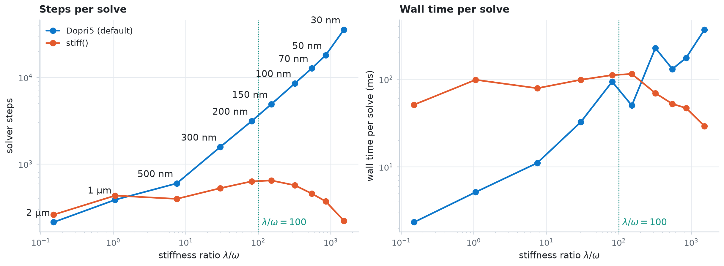
Dopri5's step count grows in proportion to \(\lambda/\omega\): it steps at the edge of its stability region, not at the accuracy it needs. The implicit Kvaerno5 solver takes a few hundred steps at any size, but each step solves a nonlinear system, so it's several times slower per step, and it compiles in seconds instead of under one. It wins the race only for the stiffest bubbles. The printed crossover depends on the machine and on what else it's running; it typically falls between \(\lambda/\omega\) of about 80 and 350.
A stiff member slows the whole batch
Under jax.vmap, as in a GridSweep, the batch runs until its slowest member finishes. One stiff bubble among easy ones makes every member wait.
steps_of = jax.jit(jax.vmap(lambda R0: solve(R0, default)[1]))
easy = jnp.full(64, 2e-6)
mixed = easy.at[-1].set(50e-9)
t_easy = wall_time(steps_of, easy, repeats=repeats)
t_mixed = wall_time(steps_of, mixed, repeats=repeats)
print(f"64 bubbles of 2 µm:                {t_easy * 1e3:6.1f} ms")
print(f"63 bubbles of 2 µm and one of 50 nm: {t_mixed * 1e3:6.1f} ms")
64 bubbles of 2 µm:                  21.4 ms
63 bubbles of 2 µm and one of 50 nm: 1632.5 ms
When the step budget runs out
A 10 nm bubble needs more than the default 100 000 Dopri5 steps. The solve stops early, the samples after that point are inf, and result.converged is False. Called outside jax.jit and jax.vmap, run_simulation also warns; inside them, check converged yourself.
tiny = lipid_bubble(R0=10e-9, freq=FREQ, pressure=100e3, cycle_num=5)
with warnings.catch_warnings(record=True) as caught:
    warnings.simplefilter("always")
    result = run_simulation(tiny.eom, tiny.pulse)
print(f"Dopri5:   converged = {bool(result.converged)}, ", end="")
print(f"{int(jnp.isinf(result.radius).sum())} of {result.radius.size} samples are inf")
for w in caught:
    print(textwrap.fill(f"warning: {w.message}", width=78, subsequent_indent="  "))

result = run_simulation(tiny.eom, tiny.pulse, config=stiff)
print(f"stiff():  converged = {bool(result.converged)}")
Dopri5:   converged = False, 113 of 1024 samples are inf
warning: ODE solver did not converge, so the trajectory is incomplete: samples
  after the failure are inf. Check `result.converged`. If the solver reached
  `max_steps`, raise `SolverConfig(max_steps=...)`, or use
  `SolverConfig.stiff()` for a stiff problem.
stiff():  converged = True
Gradients need the implicit solver
On a stiff problem, a converged Dopri5 solve can still give a useless gradient. Differentiate a loss on the radius of a 20 nm bubble with respect to the shell viscosity \(\kappa_s\). Both solvers agree on the radius, but only stiff() gives a finite gradient. Check it against a central difference of the accurate Dopri5 forward solution.
R0_SMALL = 20e-9


def loss(kappa_s, config):
    eom, pulse = lipid_bubble(
        R0=R0_SMALL, freq=FREQ, pressure=100e3, cycle_num=5, kappa_s=kappa_s
    )
    res = run_simulation(eom, pulse, save_spec=SaveSpec(num_samples=256), config=config)
    return jnp.mean((res.radius / R0_SMALL - 1.0) ** 2)


forward = jax.jit(lambda k: loss(k, default))
h = 1e-12
central = (forward(KAPPA_S + h) - forward(KAPPA_S - h)) / (2 * h)
for name, config in [("Dopri5", default), ("stiff()", stiff)]:
    t0 = time.perf_counter()
    grad = jax.jit(jax.grad(partial(loss, config=config)))(KAPPA_S)
    print(
        f"{name:8s} d loss / d kappa_s = {float(grad):+.5g}  "
        f"({time.perf_counter() - t0:.1f} s with compilation)"
    )
print(f"central difference          = {float(central):+.5g}")
Dopri5   d loss / d kappa_s = +nan  (12.7 s with compilation)
stiff()  d loss / d kappa_s = -7.2055  (20.5 s with compilation)
central difference          = -7.2056
Choosing a configuration
- Keep the default
SolverConfig()for microbubbles in water, where \(\lambda/\omega\) is below about 10: it's the fastest, both to compile and to run. - Use
SolverConfig.stiff()for nanobubbles, sub-micron bubbles in viscous liquids, and any problem with \(\lambda/\omega \gtrsim 100\), above all when you differentiate. - Check
result.converged, ordiffrax.is_successful(sol.result), whenever a solve runs underjax.jitorjax.vmap. - For a long pulse, raise
max_steps; it costs neither memory nor compile time underjax.grad. - To change the implicit solver's tolerances, call
SolverConfig.stiff(rtol=..., atol=...), so its Newton tolerances follow.